Numpy#
The original goals for the development of Python were to make it easy to read and write and flexible for many different tasks. This is reflected in the easy to use, but powerful, dynamically typed data types like lists, dictionaries. Unfortunately that same flexibility is limiting in terms of raw computational performance. For this Python relies on dedicated libraries such as Numpy which provide array-based programming idioms for fast execution of numerical calculations on data.
There are many excellent tutorials out there on Numpy. For example, a succinct beginners guide is available from the Numpy website:
Other useful user documentation and tutorials can be found here:
Here we are just going to quickly review some basic and useful aspects of numpy which will help bootstrap people for the exercises. The links above are then a useful path to do more sophisticated things. For simplicity in this quick introduction/review we will focus mostly on the 1 dimensional case, but note that the package is much more powerful than that and supports multi-dimenstional arrays.
Creating Numpy Arrays#
Numpy array can be initialized directly and explicitly as arrays:
import numpy as np

a1 = np.array([1, 2, 3, 4, 5, 6])
print(a1)
[1 2 3 4 5 6]
Dedicated functions are available to create arrays of various types:
a2 = np.ones(10)   # all ones, the function argument is the array length
print(a2)
a3 = np.zeros(10)  # all zeroes, the function argument is the array length
print(a3)
[1. 1. 1. 1. 1. 1. 1. 1. 1. 1.]
[0. 0. 0. 0. 0. 0. 0. 0. 0. 0.]
One can also create an array by specifying a first number, last number and a step size.
np.arange(start,stop,step)
Note that the rule here is “up to, but not including, the “stop” value)
a4 = np.arange(0,10,2)
print(a4)
[0 2 4 6 8]
If one wants N values linearly spaced between an initial and a final value:
np.linspace(first,last,number)
Note that in this case (unlike arange) the “last” value will be the final element.
a5 = np.linspace(0.,10,20)
print(a5)
[ 0.          0.52631579  1.05263158  1.57894737  2.10526316  2.63157895
  3.15789474  3.68421053  4.21052632  4.73684211  5.26315789  5.78947368
  6.31578947  6.84210526  7.36842105  7.89473684  8.42105263  8.94736842
  9.47368421 10.        ]
Math with Numpy Arrays#
The powerful aspect of numpy is that one can do math with these arrays. Both via scalar operations:
b1 = np.linspace(0,11,12)
print(b1)
b2 = 2*b1
print(b2)
b3 = b2 + 2
print(b3)
[ 0.  1.  2.  3.  4.  5.  6.  7.  8.  9. 10. 11.]
[ 0.  2.  4.  6.  8. 10. 12. 14. 16. 18. 20. 22.]
[ 2.  4.  6.  8. 10. 12. 14. 16. 18. 20. 22. 24.]
And via operations with different arrays (e.g. here element-wise addition):
b4 = b1 + b2
print(b4)
[ 0. 3. 6. 9. 12. 15. 18. 21. 24. 27. 30. 33.]
b5 = b4 / 3
print(b5)
[ 0. 1. 2. 3. 4. 5. 6. 7. 8. 9. 10. 11.]
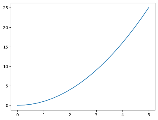
As we will see this can be useful for plotting functions, for example:
x = np.linspace(0,5,20)
y = x**2
print(x)
print(y)
[0.         0.26315789 0.52631579 0.78947368 1.05263158 1.31578947
 1.57894737 1.84210526 2.10526316 2.36842105 2.63157895 2.89473684
 3.15789474 3.42105263 3.68421053 3.94736842 4.21052632 4.47368421
 4.73684211 5.        ]
[ 0.          0.06925208  0.27700831  0.6232687   1.10803324  1.73130194
  2.49307479  3.3933518   4.43213296  5.60941828  6.92520776  8.37950139
  9.97229917 11.70360111 13.5734072  15.58171745 17.72853186 20.01385042
 22.43767313 25.        ]
import matplotlib.pyplot as plt
plt.plot(x,y)
[<matplotlib.lines.Line2D at 0x1141f3110>]
Arrays of different shapes#
The example arrays we show here are primarily one dimensional, but Numpy is a generalized package supporting multi-dimensional arrays.
(There are rules related to math with arrays of different sizes and shapes. We don’t cover that aspect here, but see the documentation links above.)
a = np.array([[0,1,2],[3,4,5]])
print(a)
print(f'The number of axes/dimensions of the array = {a.ndim}')
print(f'The shape of the array = {a.shape}')
print(f'The size of the array = {a.size}')
[[0 1 2]
 [3 4 5]]
The number of axes/dimensions of the array = 2
The shape of the array = (2, 3)
The size of the array = 6
a = np.array([[0,1,2],[3,4,5],[6,7,8]])
print(a)
print(f'The number of axes/dimensions of the array = {a.ndim}')
print(f'The shape of the array = {a.shape}')
print(f'The size of the array = {a.size}')
[[0 1 2]
 [3 4 5]
 [6 7 8]]
The number of axes/dimensions of the array = 2
The shape of the array = (3, 3)
The size of the array = 9
It is also possible to use the arange(), linspace() and other functions to create 1-dimensional arrays and then reshape them to other shapes.
a = np.arange(0,9)
print(a)
b = np.arange(0,9).reshape(3,3)
print(b)
c = np.zeros(9).reshape(3,3)
print(c)
[0 1 2 3 4 5 6 7 8]
[[0 1 2]
 [3 4 5]
 [6 7 8]]
[[0. 0. 0.]
 [0. 0. 0.]
 [0. 0. 0.]]
Accessing subsets of Numpy Arrays - “Slicing”#
An important and useful aspect of Numpy arrays is the ability to access subsets of the arrays (referred to as “slicing”) in various ways:
c1 = np.linspace(0,5,6)
print(c1)
[0. 1. 2. 3. 4. 5.]
The syntax for accessing a subset (slice) involves specifying a start index, a stop index and a step:
c1[start:stop:step]
The following rules apply:
The index numbering assigns “0” to the first element (as in C/C++, not as in FORTRAN/Julia!)
The step index is optional and assumed to be one if omitted.
If stop is specified, the elements selected will be “up to, but not including, the element at the stop index”
If the start element is not specified, elements will be included from the first element onwards.
If the stop element is not specified, elements will be included up to and including the last element
print(c1[0:2])
print(c1[:2])    # will start from first element
print(c1[0:])    # will go up to -and- include the last element
print(c1[3:])    # start with the element index 3 and go up to -and- include the last element
[0. 1.]
[0. 1.]
[0. 1. 2. 3. 4. 5.]
[3. 4. 5.]
print(c1[0:5:2]) # step by 3
[0. 2. 4.]
Negative indices can also be used, with “-1” being the last last element, “-2” the penultimate one, etc.
print(c1[3:-1]) # start with the element index 3 and go up to but not including the -1th (last) element
[3. 4.]
A negative step can be used to reverse the array:
print(c1[::-1])
[5. 4. 3. 2. 1. 0.]
Slicing with lists and strings#
Note that the slicing syntax can be applied also to other ordered data types such as lists and strings
l1 = ['apple', 'orange', 'mango', 'banana']
print(l1[0:2])
print(l1[::-1])
['apple', 'orange']
['banana', 'mango', 'orange', 'apple']
s1 = 'Abracadabra'
print(s1[0:4])
print(s1[::-1])
Abra
arbadacarbA
Masks#
Once you have a numpy array, it is also possible to select elements according to some boolean condition.
a = np.arange(0,11)
a
array([ 0, 1, 2, 3, 4, 5, 6, 7, 8, 9, 10])
b = a[a>5]   # Select only elments whose value is greater than 5
b
array([ 6, 7, 8, 9, 10])
The use of conditionals with Numpy arrays actually returns an array of boolean values whose indices correspond to the original array. A useful trick is to save this in a variable:
mask = a > 5
mask
array([False, False, False, False, False, False,  True,  True,  True,
        True,  True])
This mask can be use as the original condition was used (though as a variable it is more flexible):
c = a[mask]
c
array([ 6, 7, 8, 9, 10])
You can also use the mask to choose some elements of the array for assignment. A very useful feature is that the syntax ~mask can also be used to chose the logical not of the mask. So here for example one can use the mask to set elements greater than 5 to 5 and the ~mask to set the other elements to 0.
a[~mask] = 0
a[mask] = 5
a
array([0, 0, 0, 0, 0, 0, 5, 5, 5, 5, 5])